
Activity Feed › Discussion Forums › Strictly Surveying › How would you adjust this leveling data?
How would you adjust this leveling data?
geeoddmike replied 4 years, 6 months ago 11 Members · 33 Replies

@jim-frame
Those are post processed GPS information. We were talking about differential leveling not GPS derived orthometric elevation values.

 JS0768.The orthometric height was determined by differential leveling and
 JS0768.adjusted by the NATIONAL GEODETIC SURVEY
 JS0768.in June 1991.
- Posted by: @jt50
Those are post processed GPS information. We were talking about differential leveling not GPS derived orthometric elevation values.
Oops, I didn’t notice that network error estimates weren’t included in leveled heights. My goof.
P 1200 is one I remember in particular because in one bluebooked project I used it to validate the ortho height of another station (G 1200) in the same level line. In a previous adjustment the G 1200 height had been published based on GPS obs, and that bothered me. Once we validated (withing 2.5 cm) that G 1200 and P 1200 agreed, G 1200 got published back at its leveled height.

I thought I understood what you did but came up with different numbers. I also note that you had to reuse section difference in your approach. I am down with a cold and set up a little script to do the maths. BTW, I congratulate you on your noticing that the known points do not fit together at a high level of accuracy. For my attempt to follow your description see below:
My original post was an attempt to address the utility of the least squares method using a straightforward example. Leveling was the easiest problem I could come up with. While a previous thread dealt with GPS and least squares, that implementation is rather complex.
My work was always intended for public use and therefore the idea of “good enough” or merely giving someone a sheet of paper with values on it was insufficient. I fully accept that for in-house work and quick-and-dirty surveys; to some the rigor seems unnecessary. The fact is, a leveling adjustment following the method of least squares provides a unique, supportable solution. It is not hard to write the code to do work. It is hard to incorporate all the modeling necessary to refine the observations, convert to geopotential numbers, etc. But that’s beyond the scope of this problem.
FWIW, I copy below a heavily annotated script (using Matlab) I wrote to solve the network. I intentionally did not incorporate reading observation and other data from a file. The “%” is used to start a comment. I did not “prettify” the display units.
<<<< Matlab script follows >>>>
See: “Linear Algebra,Geodesy and GPS” by Strang and Borre
Published by Wellesley-Cambridge Press, 1997. ISBN 0-9614088-6-3
Data is from Example 8.1 pages: 286-288.
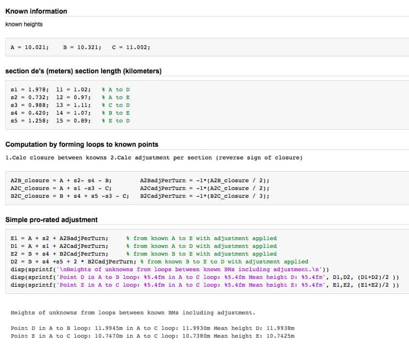
Text does not include portion related to the determination of the accuracy of the determinations. (Q matrix)Known NAVD88 heights (m) from text (vertical datum inferred): A = 10.021 B = 10.321 C = 11.002
known_H = [ 10.021; 10.321; 11.002 ];Difference in elevation (de) and section lengths (from text)
Section de (m) section length (km) A to D 1.978 1.02 A to E 0.732 0.97 C to D 0.988 1.11 B to E 0.420 1.07 E to D 1.258 0.89Create observation matrix containing de (m) and section length (km)
two column five row matrixobs = [ 1.978 1.02; 0.732 0.97; 0.988 1.11; 0.420 1.07; 1.258 0.89 ];
Stating our problem into words.
To put it into words, our equation for the first observation is: Known height A plus (+) the difference in elevation de(1) equals (=) the new height at D. More concisely: A + de(1) = D.
N.B.The values taking adjustment are the differences in elevation.
We therefore isolate the de by moving the starting BM to the right side of the equals sign. The result: de(1) = D – A
The case without a direct connection to a known height
We treat this case similarly: E + de(5) = D
Isolating the de we move E to the right side: de(5) = D – EUsing the information provided above we create an incidence matrix (Incid)
We place under the column for the point involved in the section a one(1)
or a negative one(-1).e.g. Our first observation, row one(1) is de(1) = D – A which becomes: -1 0 0 1 0 (note the -1 for A and +1 for D.
The annotated incidence matrix follows:
Sec A B C D E
———————————
1 -1 0 0 1 0 (from A to D)
2 -1 0 0 0 1 (from A to E)
3 0 0 -1 1 0 (from C to D)
4 0 -1 0 0 1 (from B to E)
5 0 0 0 1 -1 (from E to D)The Incid matrix without the annotations
Incid = [ -1 0 0 1 0 ;
-1 0 0 0 1 ;
0 0 -1 1 0 ;
0 -1 0 0 1 ;
0 0 0 1 -1 ];Reduce Incid matrix to remove columns at known heights (A,B, and C)
This becomes our design matrix A
It consists of only two columns representing the two unknowns.D E tied BM + de = preliminary H
A = [ 1 0; % 10.021 + 1.978 = 11.999
0 1; % 10.021 + 0.732 = 10.753
1 0; % 11.002 + 0.988 = 11.990
0 1; % 10.321 + 0.420 = 10.741
1 -1 ]; % + 1.258 (Not tied directly to a known BM)Compute system’s degrees of freedom (DF) from A matrix
we have five observations to determine two unknowns DF = 3
As number rows = number of observations and number of columns = number of stations use size() function to report dimensions then subtract them.[a,b] = size(A); % dimensions of design matrix
DF = a – b; % DF = degrees of freedomReduced observation matrix (L) reflecting direct ties to known BMs (see above)
L = [ 11.999;
10.753;
11.990;
10.741;
1.258 ];Create preliminary weight matrix
W = ones(5,1) ./ obs(:,2); % weight is inverse of section length
P = diag(W); % weights on diagonal of 5 x 5 matrix
Solve for heights at unknowns and residualsUsed inverse function (inv) here due to issues related to my using the latest MacOS and my old version of Matlab.
Should use X = P*A P*L, the left division operatorSolve for unknown heights and observation residuals
X = inv(A’*P*A)*(A’*P*L); % solves for unknown heights
V = A*X – L; % calculates observation residuals
% in sense computed – observed (Strang and Borre use V = L -A*X)
Solution statisticsVAR = (V’*P*V)/DF; % solve for variance of unit weight (VUW)
STDEV = sqrt(VAR); % solve for standard deviation
Q = inv(A’*P*A); % weighted design matrix
VCV = STDEV * Q; % variance-covariance matrixSince the weights were not correct given the non unitary VUW additional work is necessary. NOT DONE HERE.
To prove the determined X is optimal
add 0.0001 m to heights at unknowns then resolve for residuals
Xtest = X + [ 0.0001; 0.0001 ]; % add a mm to computed heights (in X)
Vtest = A * Xtest – L; % variances with test X
diff_in_Vsqrd = sum(V .* V) – sum(Vtest .* Vtest);
Outputssprintf(‘nSolved heights for unknownsnD = %5.4f mtE = %5.4f m’, X(1),X(2))
sprintf(‘nObservation and residualsn’)
disp([L V])
sprintf(‘nVariance of Unit Weight: %5.4f’, VAR )
sprintf(‘nStandard deviation: %5.4f’, STDEV )
sprintf(‘nWe add a tenth millimeter to solved heights for testing.’)
disp(Xtest)
sprintf(‘nComputed residuals using these test heights.’)
disp( [L Vtest])
sprintf(‘nThe principle of least squares is that the correct answer is the one where the sum of squares of the errors is a minimum.’)
sprintf(‘nWe prove our computed answer is the best by comparing the sum of variances.’)
sumV_sqrd = V’*V;
sumVtest_sqrd = Vtest’ * Vtest;Solved heights for unknowns (displayed to four decimal places)
D = 11.9976 m E = 10.7445 m
Observation and residuals
11.999 -0.00138986387474738
10.753 -0.00850076737886774
11.99 0.00761013612525296
10.741 0.00349923262113272
1.258 -0.00488909649587921Variance of Unit Weight: 0.0001
Standard deviation: 0.0075
We add a tenth millimeter to solved heights for testing.
11.9977101361253
10.7445992326211Computed residuals using these test heights.
11.999 -0.00128986387474761
10.753 -0.00840076737886797
11.99 0.00771013612525273
10.741 0.00359923262113249
1.258 -0.00488909649587921The principle of least squares is that the correct answer is the one where the sum of squares of the errors is a minimum.
We prove our computed answer is the best by comparing the two sums of variances.
if sumV_sqrd < sumVtest_sqrd
sprintf(‘nSum of V^2 squared is smaller than heights altered by 1 mm.’)
else
sprintf(‘nSum Vtest V^2 is smaller than using computed heights.n’)
endSum of V^2 squared is smaller than heights altered by 1 mm.
end of file

GeeOddMike I have been following your post and reading the comments and would like to add
some comments myself. #1, its to bad you had an error in labeling one of the points. It seems to have
taken away form your post (a little). #2, Your very first question was “How would you derive heights
for the unknown points…”; The very first thing I thought of was “Manual of Leveling Computation
and Adjustment by Rappleye , Special Pub. 240 USC&GS 1948.
No place in your post did you ask for something other than a Least Squares Adj.; this came later.
When you did ask for something other than LSA then I thought of the “DELL ADJ.”
The Dell method is in the references of “Surveying Theory and Practice by Davis, Foote and Kelley” page
212 of the 5th edition. A better place to look is in “Surveying for Civil Engineers by Prof. Kissam, 2nd edition
chapter 6, starting on page 156 (a worked example is given). Two other places you can find H.G. Dell method
are both in ASCE; Vol. 61, no. 4, April 1935 (part 1) and same journal Vol. 101, pp. 834-856, 1936. (part 2)
I have had Dr. Strang book since it was published and find it very good.
JOHN NOLTON
Thanks for the references. While “ancient” Rappleye’s manual is still useful.
My efforts to get those instinctively opposed to considering least squares to at least recognize its value remain unsuccessful.
I too like the Strang/Borre text. Prof Strang’s linear algebra course is available for viewing at: https://ocw.mit.edu/courses/mathematics/18-06-linear-algebra-spring-2010/video-lectures/ He is a good communicator. I had the pleasure of attending one of his lectures.
Given the inattention paid to the monumented vertical network, these monuments have diminished in numbers and not updated to reflect geophysical and other changes. This hinders efforts like the GPS on BM program as an earlier thread on efforts to resolve possible geoid modeling errors in the Scranton, PA area. It seems that many considered work on the nationwide leveling network to have been finished with NAVD88.
As for leveling adjustments, the image file below describes how one goes about determining the accuracy of a leveling project. Note that this FGCS document has much more information on the data acquisition and observation phases. See: https://www.ngs.noaa.gov/FGCS/tech_pub/Fgcsvert.v41.specs.pdf
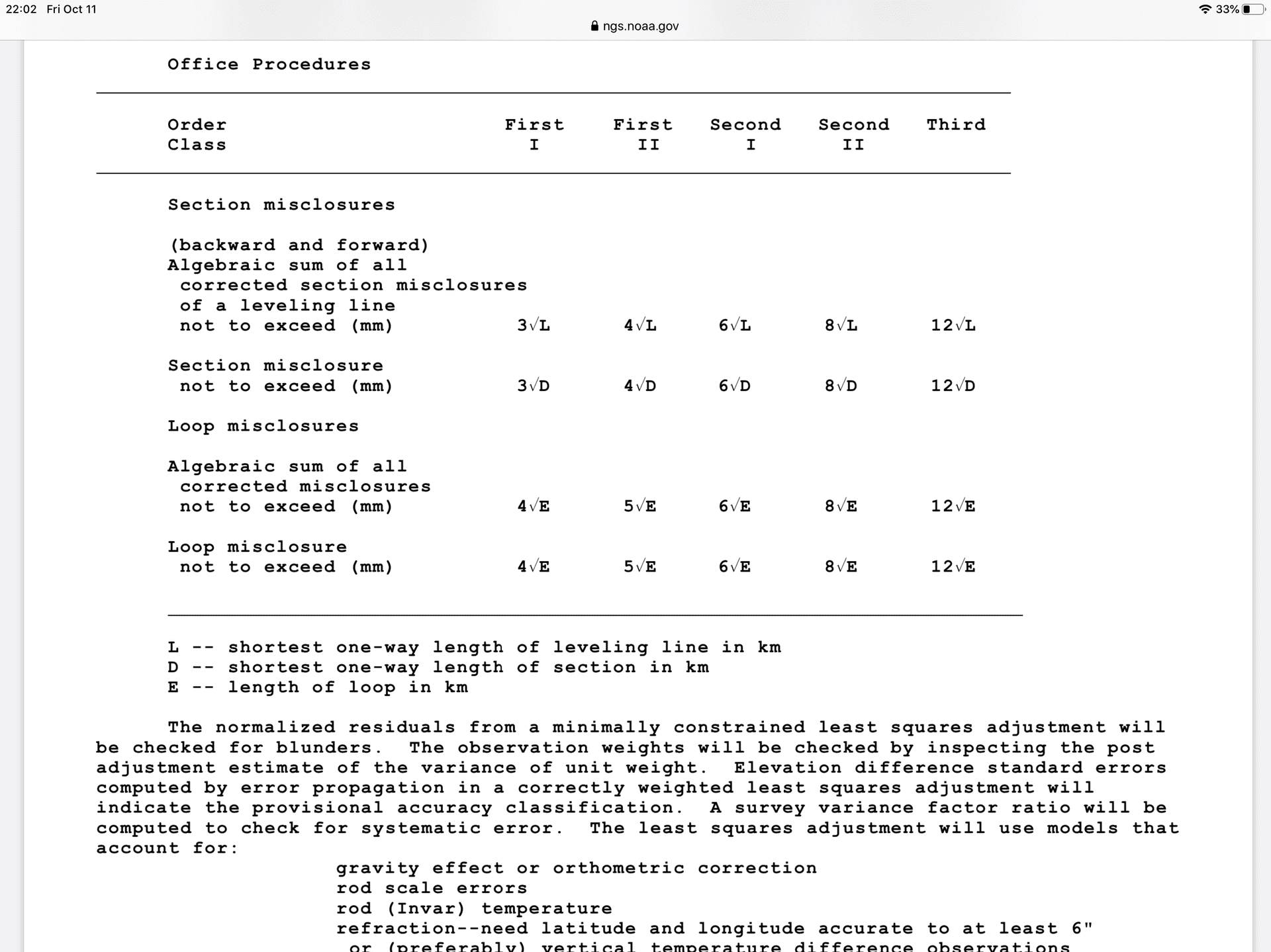

This exercise, in my mind, is designed for a hand calculation of a least squares adjustment of the data in a classroom setting. The pedagogical value is in seeing how observations are turned into equations, how redundant observations are incorporated, and how results are obtained by applying maxima/minima principles from the calculus. Duplicating the answers from a black box removes some of the mystery from the black box.
So let’s go through the exercise and see if there’s anything to be learned.
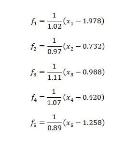
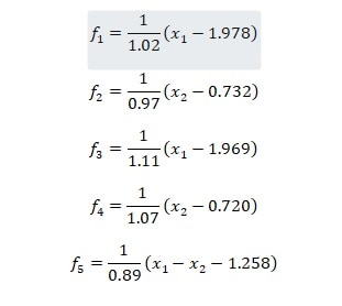
Here are the observation equations, written in the form of the least-squares adjustment to be made to each difference in elevation. Note that the reciprocals of the lengths of the segments are used to weight the differences. This adjusts a shorter length more than a longer one.
We only want values for two items, the heights of D and E, yet we have five equations. Let’s look for redundancies; equations that can be derived from one of the other equations. Here’s how we do that.
1. We want the height of E to be the same value whether we compute it from B or from A.
2. We want the height of D to be the same value whether we compute it from C or from A.
3. We want the value of the change in height between D and E to be the same whether we compute it from D to E or from E to D. (Note: This will not be true if simple averages of AE and BE, and AD and CD are used for the heights of E and D, respectively.)
Here are the condition equations that describe these conditions:
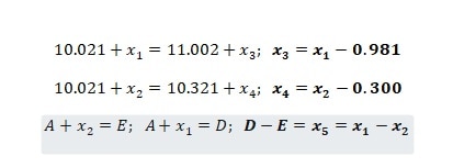
Substituting the condition equations into the appropriate observation equations gives these new equations:
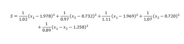
Since it is the sum of the differences squared that we want to minimize, we need an equation that sums up the differences squared:
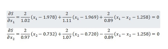
Now for the calculus. The principle is that, when a function is minimized, its first derivative is 0. In the case of multi-variable functions (our sum function has two variables) each of the partial derivatives is 0 when the function is minimized. Here are the partial derivatives:
We now have two equations in two unknowns, but they need to be simplified:
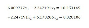
Solving these equations and substituting appropriately produces the following values:
x1 = 1.976610
x2 = 0.723499
x3 = 0.99561
x4 = 0.423499
x5 = 1.253111
D = 11.998
E = 10.744
These are the best estimates for D and E because they resolve the three readily-identifiable ambiguities in a non-arbitrary way. As to the accuracy, that requires a separate analysis and statistical assumptions that may not be met in the problem.
Well, that was a lot of work. I learned a great deal from doing it and I hope you did, too.

E= 10.740
D (F) = 11.991
I did not use any software, I did not use least squares. I just used common sense and a calculator. It took about 4 minutes. If I average to two separate runs from E to D, I get 1.252. Calculating from B to C using 1.252 for the middle run I get .003 mm error at C. I distributed that error .001 mm for each of the three runs.
How Accurate? I don’t know, I didn’t run it but for the type of work I do, it is plenty good. If I was setting new permanent monuments, I would rerun it.
Prove your answer is the best possible? I can’t do that. but it is good enough for me and that is all that counts.
James
- Posted by: @jaro
I did not use any software, I did not use least squares.
That works great when you have a handful of turns and a few marks to deal with. Try it with tens of km of leveling and dozens of marks and the error propagation is much more difficult to properly model.

Surely part of being a professional is knowing when to keep it simple and when to use a more elaborate method?
Just trying to learn. Aren’t there 4 different paths through E-D, two starting at A, one from B and one from C? Why did you choose A-E-D-A and B-E-D-A instead of some other pair?

I knocked on the door of Prof Strang’s house and bought, face-to-face, a copy of his “Linear Algebra, Geodesy, and GPS” book when it came out. ???? I think I did phone first to make sure he’d be home. He was very nice about it!
The Cambridge-Wellesley Press is certainly an old-fashioned enterprise. Ordering involves sending an email to Prof Strang??s email. No credit cards; personal service. Sounds like a positive experience.
I was under the impression the ??Linear Algebra, Geodesy and GPS? text was out of print. It is still listed among the Press?? catalog. See: http://www-math.mit.edu/~gs/books/catalog.html
I failed to mention that there are a number of Matlab script files associated with the text that are available for free download at: http://www.i4.auc.dk/Borre/Matlab
His Matlab tools for GPS are here: http://kom.aau.dk/~borre/life-l99/ I did not like the ??Algorithms in Global Positioning?? text as much.
For those unwilling to pay for a copy of Matlab, try Scilab. It is free and comparable to Matlab in many ways. See: https://www.scilab.org/
BTW an Amazon search for the text shows only used copies available with asking prices as high as these:


Log in to reply.